# Using Multiverse in a Jupyter Notebook

Prototyping is an essential step in software development. When it comes to prototyping Python code for Maya we usually end up using one of these two choices:

The Maya Script Editor
The Maya Python interpreter

The Maya Script Editor allows us to run Python code directly in the Maya UI while the the Maya Python interpreter works as a proper interpreter with all the advantages and disadvantages of such approach (e.g. hard to navigate through the code and re-run some parts).

In this post we'll introduce an alternative way to run Python code for Maya that takes an approach in between a full UI session and a raw interpreter: using Jupyter Notebook.

# What's Jupyter Notebook

Jupyter Notebook (opens new window) is an open-source web application that allows users to create documents that contain live code along with text (using Markdown) and graphics (for example for data visualization). Jupyter Notebook is part of the Jupyter project (opens new window) and supports multiple programming languages, including Python, R, Julia, etc. Notebooks can be created online (see https://jupyter.org/try (opens new window)) or locally and can be saved and shared with other users.

# Installing Jupyter Notebook

The easiest way to try out Jupyter Notebook is to install it into a Python virtualenv (opens new window). Assuming pip (opens new window) is installed in our system, we can install virtualenv using:

pip install virtualenv

Note

Make sure you install virtualenv for Python 2.7 since that's the version of the interpreter shipped with Maya 2018, 2019 and 2020.

Let's start with creating a new environment called multiverse:

> cd /path/to/my/envs
> virtualenv multiverse

1
2

This command will create a new multiverse sub-folder and will populate it with a basic folder structure:

multiverse/
|-- bin
|-- include
|-- ...
`-- lib

1
2
3
4
5

This folder represents our virtual Python environment and will allow us to install Python modules in a scoped way, without affecting the system.

New environments are not active by default, to activate our multiverse environment run:

> cd multiverse/
> source bin/activate

1
2

Your prompt should now show the name of the active environment (multiverse in our case):

(multiverse) >

1
2

Now that our environment is set up and active, we can install Jupyter:

(multiverse) > pip install jupyter

# Adding a Maya Python kernel

In Jupyter, kernels (opens new window) are processes that run independently and interact with the Jupyter applications and their user interfaces. Many kernels (opens new window) are available for Jupyter, but for our use case we'll define a custom kernel that uses Maya's Python interpreter. Kernels are stored as .json files in the share/jupyter/kernels folder. Since we're using a virtual environment, we'll create our kernel in the multiverse environment folder:

(multiverse) > cd /path/to/my/envs/multiverse
(multiverse) > cd share/jupyter/kernels

1
2

Here we would need to create a sub-folder for our kernel and create a kernel.json file in it:

(multiverse) > mkdir mayapy_2019
(multiverse) > vim mayapy_2019/kernel.json

1
2

The content of the kernel file is shown below, change the display_name and the path of the Maya Python interpreter according to your platform and the version you want to use:

{
  "display_name": "Maya 2019",
  "language": "python",
  "argv": [
    "/usr/autodesk/maya2019/bin/mayapy",
    "-m",
    "ipykernel_launcher",
    "-f",
    "{connection_file}"
  ]
}

1
2
3
4
5
6
7
8
9
10
11

# Running Jupyter Notebook

Before running Jupyter let's create a folder where all our notebooks will be stored (notebooks use the.ipynb extension).

(multiverse) > cd /path/to/my/envs/multiverse
(multiverse) > mkdir notebooks

1
2

Move into the notebooks folder and start Jupyter using:

(multiverse) > cd notebooks
(multiverse) > jupyter notebook

[I 12:31:59.672 NotebookApp] Serving notebooks from local directory: /path/...
[I 12:31:59.672 NotebookApp] The Jupyter Notebook is running at:
[I 12:31:59.672 NotebookApp] http://localhost:8888/?token=efbb0669db003...
[I 12:31:59.672 NotebookApp] Use Control-C to stop this server and shut down all
    kernels (twice to skip confirmation).
...

1
2
3
4
5
6
7
8
9

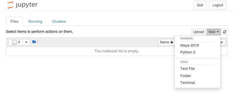
Jupyter Notebook will start a local http server and automatically open its welcome page in your default browser.

Here we can create our first notebook by clicking the New button and selecting the Maya 2019 notebook type that will run our custom kernel.

At this point we can create a new cell and start evaluating our code in the Jupyter Notebook's web interface (refer to the Jupyter Notebook user guide (opens new window) for details about commands and shortcuts).

First of all let's make sure the Maya interpreter is correctly initialized using:

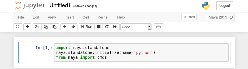
Here's the code showed in the image above for reference:

import maya.standalone
maya.standalone.initialize(name='python')
from maya import cmds

1
2
3

Once the interpreter is initialized we can load the Multiverse plug-in and import the multiverse Python module:

maya.cmds.loadPlugin('MultiverseForMaya')

import multiverse as mv

1
2
3

As a first example let's load a USD asset with the Multiverse API and query the asset paths:

node = mv.CreateUsdCompound('/tmp/cube.usda')
print(node)

paths = mv.GetUsdCompoundAssetPaths(node)

1
2
3
4

Here's an image of our notebook with all the code in the cells begin evaluated.

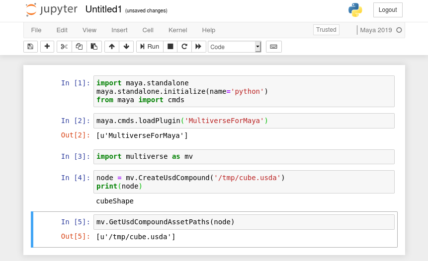
Notice that when a cell is evaluated the result of the last statement, if any, is automatically printed in the cell's output.

You can now carry on from this example or create other notebooks to continue prototyping your code through the intuitive and interactive Jupyter Notebook web interface.

Happy prototyping with Multiverse and Jupyter Notebook!